Advanced GEMM Optimization on Modern x86-64 Multi-Core Processors

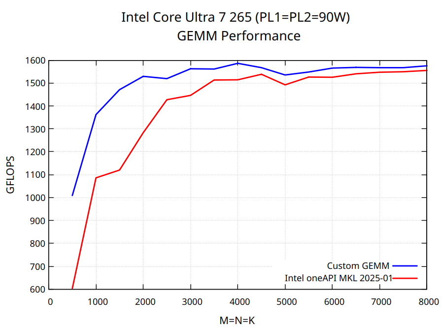
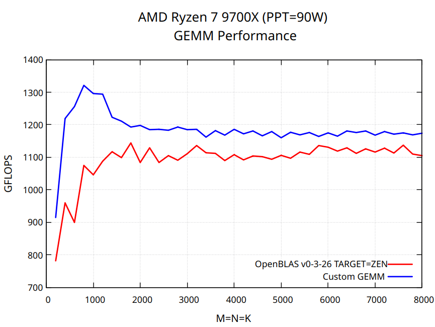
TL;DR The code is available at matmul.c. This blog post demonstrates how to optimize multi-threaded FP32 matrix multiplication for modern processors using FMA3 and AVX2 vector instructions. The optimized custom implementation resembles the BLIS design and outperforms existing BLAS libraries (including OpenBLAS and MKL) on a wide range of matrix sizes. This implementation shows strong performance across various x86-64 architectures, both in single-threaded and multithreaded settings. However, achieving optimal speed requires careful adjustment of hyperparameters e.g. the number of threads, kernel size, and tile sizes. Additionally, on AVX-512 CPUs, the BLAS libraries might be notably faster due to AVX-512 instructions, which were intentionally omitted here to support a broader range of processors. The achieved performance on AMD Ryzen 7 9700X is shown below.

P.S. Please feel free to get in touch if you are interested in collaborating. My contact information is available on the homepage.

1. Introduction

Matrix multiplication is an essential part of nearly all modern neural networks. Despite using matmul daily in PyTorch, NumPy, or JAX, I’ve never really thought about how it is designed and implemented internally to take full advantage of hardware capabilities. NumPy, for instance, relies on external BLAS (Basic Linear Algebra Subprograms) libraries. These libraries contain high-performance, optimized implementations of common linear algebra operations, such as the dot product, matrix multiplication, vector addition, and scalar multiplication. Examples of BLAS libraries include:

Intel MKL - optimized for Intel CPUs
Accelerate - optimized for Apple CPUs
BLIS - open-source, multi-vendor, BLAS-like Library Instantiation Software
GotoBLAS - open-source, multi-vendor
OpenBLAS - open-source, multi-vendor, fork of GotoBLAS

A closer look at the OpenBLAS code reveals a mix of C and low-level assembly. In fact, OpenBLAS, GotoBLAS, and BLIS are written in C/FORTRAN/Assembly and contain matmul implementations manually optimized for different CPU microarchitectures. My goal was to implement the matrix multiplication in pure C (without low-level assembly code) so that it works for any matrix size, runs on all modern x86-64 processors, and competes with existing BLAS libraries. At the sime time I wanted to keep the code simple and easy to extend. After some research, I found a few great step-by-step tutorials on implementing fast matrix multiplication from scratch, covering both theory and practice:

Fast Multidimensional Matrix Multiplication on CPU from Scratch by Simon Boehm.
Matrix Multiplication by Sergey Slotin.
Geohot’s stream Can you multiply a matrix?

I highly recommend these clear and well-explained tutorials with alternative implementations. They helped me better understand the topic and, in some sense, motivated me to write my own implementation. The reason is that all three solutions above work only for specific matrix sizes and do not achieve performance of the BLAS libraries. Unsatisfied with these results, I kept researching and came across two fascinating papers: “Anatomy of High-Performance Matrix Multiplication” and “Anatomy of High-Performance Many-Threaded Matrix Multiplication”. The first introduces GotoBLAS, a high-performance BLAS implementation by Kazushige Goto. The second reviews the matmul design used in the BLIS library (an extended version of GotoBLAS) and explores different parallelization strategies. Due to its superior high-level design, I had a feeling that the matmul implementation from the BLIS library can outperform existing BLAS implementations even if written in pure C and not manually finetuned using inline assembly. In the next chapters we’ll step-by-step implement the algorithm from scratch and compare against OpenBLAS. Before diving into optimizations, let’s first go over how to install OpenBLAS and properly benchmark the code on a CPU.

2. How to Install and Benchmark OpenBLAS

I benchmarked the code on the following machine:

CPU: AMD Ryzen 7 9700X
RAM: 32GB DDR5 6000 MHz CL36
OpenBLAS 0.3.26
Compiler: GCC 13.3
Compiler flags: -O3 -march=native -mno-avx512f -fopenmp
OS: Ubuntu 24.04.1 LTS

Important! To obtain reproducible and accurate results, minimize the number of active tasks, particularly when benchmarking multi-threaded code. Windows systems generally deliver lower performance compared to Linux due to higher number of active background tasks.

To benchmark OpenBLAS, start by installing it according to the installation guide. During installation, make sure to set an appropriate TARGET and disable AVX512 instructions for a fair comparison. For Zen4/5 processors compile OpenBLAS with:

make TARGET=ZEN

Otherwise, OpenBLAS defaults to AVX512 instructions. After installation, you can run FP32 matmul using the OpenBLAS API:

#include <cblas.h>
cblas_sgemm(CblasColMajor, CblasNoTrans, CblasNoTrans, m, n, k, 1, A, m, B, k, 0, C, m);

The benchmark evaluates the custom implementation and the OpenBLAS API on square matrices, ranging from m=n=k=200 to m=n=k=10000 in steps of 200. To obtain consistent and accurate results, matrix multiplication is repeated n_iter times, and performance is measured as median execution time.

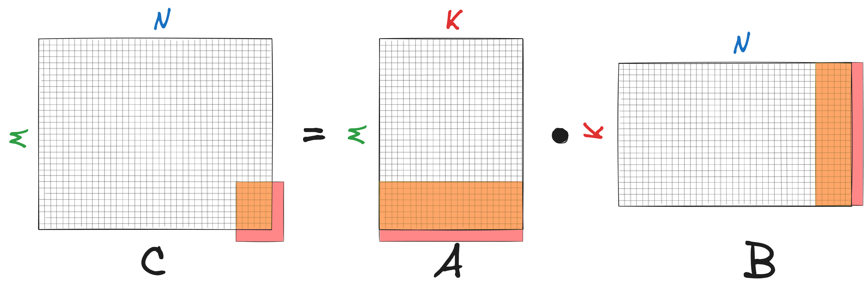
To multiply two float32 matrices - $A$ of size $M \times K$ and $B$ of size $K \times N$, for each element of the resulting matrix $C$ of size $M \times N$, we need to compute the dot product between a row of $A$ and a column of $B$. This requires $K$ (additions) + $K$ (multiplications) = $2K$ Floating Point Operations (FLOP) per element of $C$ or $2MNK$ FLOP in total. A metric often used to evaluate matmul performance is called FLOP per second or FLOP/s or FLOPS, and it can be derived from the execution time as FLOPS=FLOP/exec_time=(2*m*n*k)/exec_time.

3. Theoretical Limit

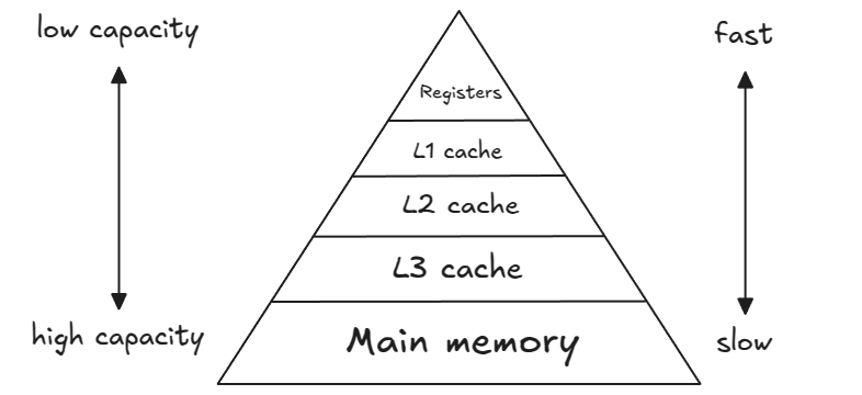
The image below shows a simplified model of the computer’s memory hierarchy (for now, ignore the layers between the registers and the main memory(=RAM); we will discuss them later).

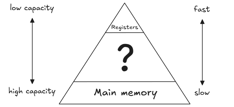
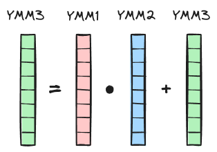
To perform arithmetic operations on data stored in RAM (off-chip memory, slow and large capacity), the data must be first transferred to CPU and placed in CPU registers (on-chip memory, fast and small capacity). Modern x86-64 CPUs support SIMD (Single Instruction Multiple Data) extensions, which allow multiple pieces of data to be processed in parallel. There are various SIMD extensions, but the ones relevant to our discussion are Advanced Vector Extensions (AVX2) and Fused Multiply-Add (FMA). Both AVX2 and FMA operate on data stored in special 256-bit YMM registers. Each YMM register can hold 8 packed single-precision (32-bit) floats. The FMA2 instructions perform element-wise multiply-add operation on data stored in the YMM registers. The corresponding assembly instruction is called VFMADD231PS (PS stands for PackedSingle) and takes three vector registers (YMM1, YMM2, YMM3) as input to compute YMM1 = YMM2 * YMM3 + YMM1.

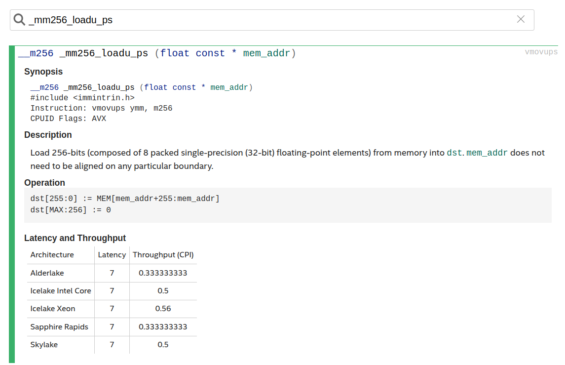
According to the intel intrinsics guide or https://uops.info/table.html, for my CPU the throughput (TP) of the fused-multiply-add instruction is 0.5 cycles/instruction or with other words 2 instructions/cycle:

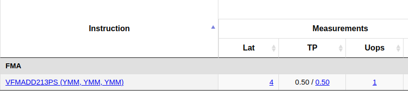
Theoretically, Ryzen 9700X can perform 32 FLOP per cycle: 8 (floats in YMM register) * 2 (add + mul) * 2 (1/TP). Therefore, the theoretical peak FLOPS in single-threaded mode can be roughly estimated as CPU_CLOCK_SPEED * 32 or n_cores * CPU_CLOCK_SPEED * 32 in multi-threaded mode. For example, assuming a sustainable clock speed of 4.7 GHz for an 8-core 9700X processor, the theoretical peak FLOPS in a multi-threaded setting would be 1203 FLOPS.

4. Naive Implementation

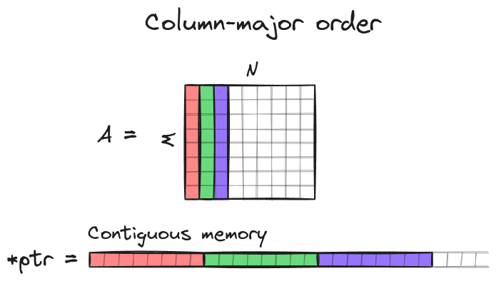
In this tutorial we assume that matrices are stored in column-major order: e.g. matrix A of shape MxN is stored as contiguous array of length M*N and an element A[row][col] is accessed via C raw pointer ptr[col*M + row], where 0 <= col <= N-1 and 0 <= row <= M-1.

The simplest implementation of $C=AB$ can be described as follows:

void matmul_naive(float* A, float* B, float* C, const int M, const int N, const int K) {
  for (int i = 0; i < M; i++) {
    for (int j = 0; j < N; j++) {
      for (int p = 0; p < K; p++) {
        C[j * M + i] += A[p * M + i] * B[j * K + p];
      }
    }
  }
}

Here, we iterate over all rows (the outermost loop) and all columns (the second loop) of C and for each element of C we calculate the dot product (the innermost loop) between the corresponding row of matrix A and column of matrix B. It’s always good to start with a simple and robust algorithm that can later be used to test optimized implementations.

5. Kernel

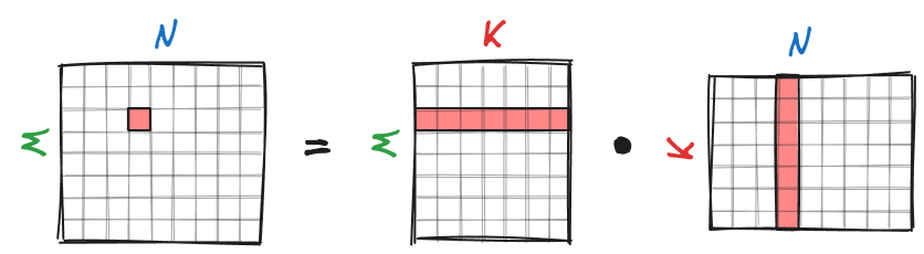
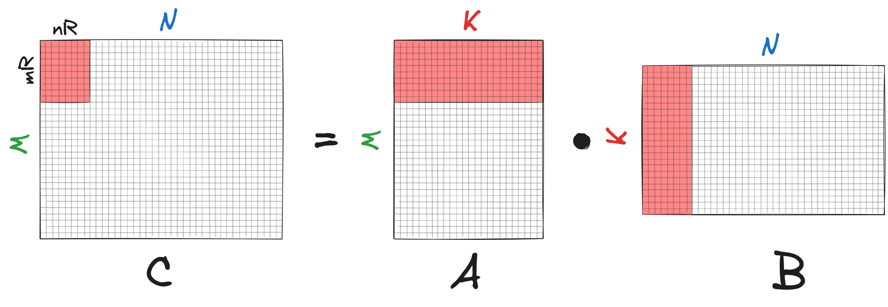
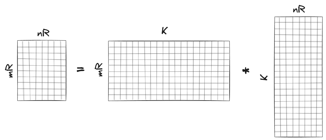
The key idea of high-performance matrix multiplication on CPU is to develop a function that efficiently computes a sub-matrix of $C$. Then, by iterating over $C$ and applying this function to all non-overlapping sub-matrices, we can significantly speed up the entire matrix multiplication operation. For this, we, first, partition the matrix $C$ of shape $M \times N$ into smaller non-overlapping sub-matrices of shape $m_R \times n_R$, with $n_R \ll N$ and $m_R \ll M$. To calculate $C=AB$, we iterate over $C$ and compute each of its non-overlapping $m_R \times n_R$ sub-matrices as shown below:

The function that computes an $m_R \times n_R$ sub-matrix $\bar{C}$ of $C$ is called a kernel (aka. micro-kernel using BLIS notation). This function is the core of high-performance matrix multiplication. When we say a matrix multiplication algorithm is optimized for a specific CPU architecture, it usually refers to kernel optimization. For example, OpenBLAS contains kernels optimized for different CPU microarchitectures.

Let’s take a closer look at the kernel. To compute an $m_R \times n_R$ sub-matrix $\bar{C}$ of $C$, we need to multiply corresponding $m_R \times K$ sub-matrix $\bar{A}$ of $A$ with $K \times n_R$ sub-matrix $\bar{B}$ of $B$ as shown in the figure below:

If we were to do this in a naive manner using the dot product, we would need to fetch $2K$ elements from RAM to calculate a single element of $\bar{C}$ or $2K m_R n_R$ elements in total to compute $\bar{C}$. There is, however, an alternative strategy that can reduce the number of fetched elements.

First, we initialize the matrix $\bar{C}$ with zeros and store it in registers. Since both $n_R$ and $m_R$ are small, the entire matrix fits within the registers. Here, the subscript $R$ in $n_R$ and $m_R$ denotes “register”. Next, we iterate over the dimension $K$, and in each iteration, we:

load 1 column of $\bar{A}$ and 1 row of $\bar{B}$ from RAM into the registers. Again, note that both the row and column vectors are limited in size and can be stored in the registers.
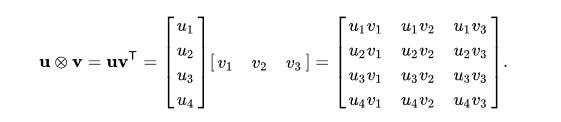
compute the outer product between the two vectors and add the result of the outer product to the matrix $\bar{C}$.

After $K$ iterations, the computation of the matrix $\bar{C}$ is completed and it can be stored into RAM. $\bar{C}$ is often referred to as the accumulator, because it accumulates the outer products along the dimension $K$. A single accumulation step of the outer product between two vectors is also known as rank-1 update.

Outer product between a column vector and a row vector.

In total, we fetch $(m_R + n_R)K$ elements from RAM into registers. Compared to the naive approach, this reduces the number of memory accesses by a factor of

\[\frac{2m_Rn_RK}{(m_R + n_R)K} = \frac{2m_Rn_R}{m_R + n_R}\]

This factor is maximized when both $m_R$, $n_R$ are large and equal. However, the values of $m_R$ and $n_R$ are typically constrained by the available register memory.

Now, let’s discuss in detail how the outer product and accumulation can be efficiently implemented using SIMD FMA instructions. Unfortunately, there are no SIMD instructions that compute the outer product in a single step. Therefore, we need to decompose the outer product into simpler operations. The figure below illustrates the process:

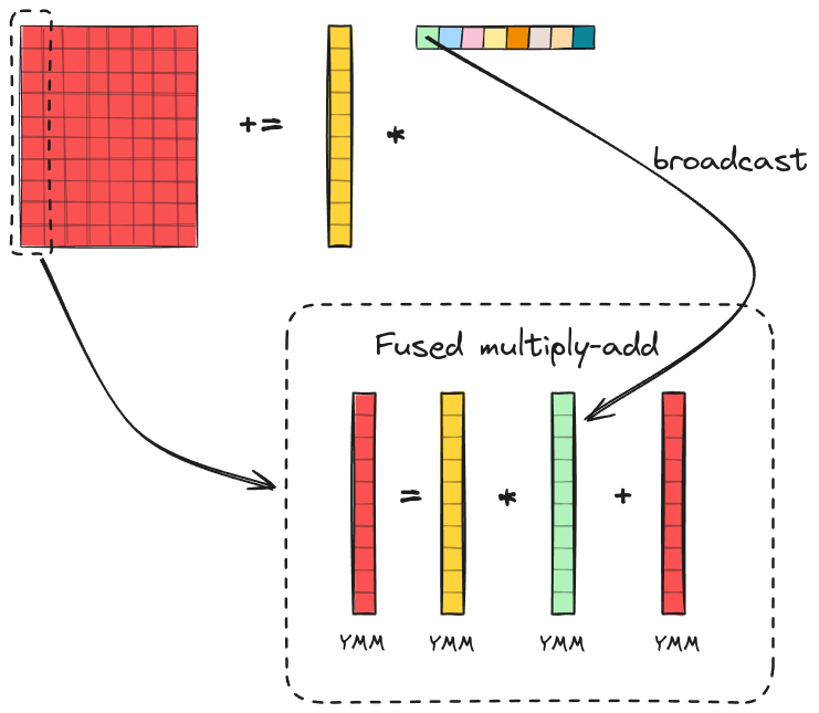
Here, we compute the outer product between a column vector of size $m_R$ and a row vector of size $n_R$ to update an accumulator $\bar{C}$ of size $m_R \times n_R$. The accumulator is stored in the YMM registers, with each column of the accumulator spanning one or multiple YMM registers. The column vector is also stored in the YMM registers (highlighted as yellow). Since each YMM register holds 8 floats, the dimension $m_R$ must be divisible by 8. The accumulator is updated column by column. During the first iteration we broadcast the first element of the row vector to a vector of size $m_R$ and place it in the YMM registers (highlighted as green). Then, we element-wise multiply the column vector with the broadcasted vector and accumulate the result to the first column of the accumulator $\bar{C}$ using FMA instruction. We repeat this process for the remaining elements of the row vector to update the corresponding columns of the accumulator. After $n_R$ iterations, the rank-1 update of the accumulator is completed.

The last thing we need to discuss before implementing the kernel in C is how to choose the kernel size i.e. $m_R$ and $n_R$. CPUs with AVX support have 16 YMM registers. From our previous discussion, we know that we need $(m_R/8) \cdot n_R$ registers to store the accumulator $\bar{C}$, $m_R/8$ registers to store the column vector and 1 register (because we can reuse the same register for all FMA operations) for the broadcasted vector. We want $m_R$ and $n_R$ to be as large as possible while satisfying the following conditions:

$\Big(\cfrac{m_R}{8} \cdot n_R + \cfrac{m_R}{8} + 1\Big) <= 16$
$m_R$ is a multiple of 8

In theory we want $m_R = n_R$ to minimize the number of fetched elements. However, in practice, a non-square kernel with $m_R = 16, n_R = 6$ showed the best performance on my CPU. Therefore, we will implement this kernel in the next section. Feel free to experiment with other kernel sizes, such as $8 \times 8, 8 \times 12$, $8 \times 13$, $8 \times 14$, $32 \times 2$ and compare their performance on your CPU.

Let’s implement the algorithm discussed above using the $16 \times 6$ kernel. The code of this implementation can be found at matmul_kernel.c. To use SIMD instructions in C we first need to include the immintin.h library:

#include <immintrin.h>

The implementation of the algorithm is straightforward: we iterate over matrix $C$ and apply the kernel function to each of it’s non-overlapped $16 \times 6$ sub-matrices $\bar{C}$.

void matmul_kernel(float* A, float* B, float* C, const int M, const int N, const int K) {
  for (int i = 0; i < M; i += 16) {
    for (int j = 0; j < N; j += 6) {
        kernel_16x6(&A[i], &B[j * K], &C[j * M + i], M, N, K);
    }
  }
}

The kernel function is declared as follows:

void kernel_16x6(float* A_start, float* B_start, float* C_start, int M, int N, int K);

The function takes as input pointers to the starting positions of $\bar{A}, \bar{B}$, and $\bar{C}$ along with the matrix problem size. It then computes $16 \times 6$ sub-matrix $\bar{C}$ of $C$ according to $\bar{C} = \bar{A} \bar{B}$.

Inside the kernel function, first, we declare the variables stored in the YMM registers:

__m256 C_accum[6][2] = {}; // zero-initialized
__m256 b_packFloat8;
__m256 a0_packFloat8;
__m256 a1_packFloat8;

A variable of type __m256 is a 256-bit vector that represents the contents of a YMM register, which holds eight 32-bit floating-point values. C_accum is the accumulator stored in the YMM registers. The variable b_packFloat8 contains a broadcasted element from a row vector of $\bar{B}$, while a0_packFloat8 and a1_packFloat8 represent a column vector of $\bar{A}$. Since the column vector contains 16 floats, it requires two YMM registers for storage.

SIMD intrinsics are well documented and can be found in the Intel Intrinsics Guide. For example, _mm256_loadu_ps

The kernel iterates over the dimension $K$ and in each iteration performs a rank-1 update of the accumulator:

for (int p = 0; p < K; p++) {
  // Load column vector of size 16
  // {
  a0_packFloat8 = _mm256_loadu_ps(&A_start[p * M]);
  a1_packFloat8 = _mm256_loadu_ps(&A_start[p * M + 8]);
  // }
  // Broadcast scalar element to vector of size 8
  // {
  b_packFloat8 = _mm256_broadcast_ss(&B_start[p]);
  // }
  // Update the first column of the accumulator
  // {
  C_accum[0][0] = _mm256_fmadd_ps(a0_packFloat8, b_packFloat8, C_accum[0][0]);
  C_accum[0][1] = _mm256_fmadd_ps(a1_packFloat8, b_packFloat8, C_accum[0][1]);
  // }
  ...
  ...
  ...
  b_packFloat8 = _mm256_broadcast_ss(&B_start[5 * K + p]);
  // update the last column of the accumulator
  // {
  C_accum[5][0] = _mm256_fmadd_ps(a0_packFloat8, b_packFloat8, C_accum[5][0]);
  C_accum[5][1] = _mm256_fmadd_ps(a1_packFloat8, b_packFloat8, C_accum[5][1]);
  // }
}

After $K$ rank-1 updates, the computation of the accumulator is complete, and the result can be stored in RAM:

// Store the accumulator column by column:
for (int j = 0; j < 6; j++) {
  _mm256_storeu_ps(&C_start[j * M], C_accum[j][0]);
  _mm256_storeu_ps(&C_start[j * M + 8], C_accum[j][1]);
}

Let’s take a look at the generated assembly code to see if it actually contains SIMD FMA instructions and uses the YMM registers:

gcc -O3 -mno-avx512f -march=native matmul_kernel.c -S

// matmul_kernel.s
...
vfmadd231ps	%ymm14, %ymm1, %ymm13
vfmadd231ps	%ymm14, %ymm0, %ymm12
vmovaps	%ymm13, 32(%rsp)
vmovaps	%ymm12, 64(%rsp)
vbroadcastss	(%rax,%r9), %ymm14
vfmadd231ps	%ymm14, %ymm1, %ymm10
vfmadd231ps	%ymm14, %ymm0, %ymm11
vmovaps	%ymm10, 96(%rsp)
vmovaps	%ymm11, 128(%rsp)
vbroadcastss	(%rax,%r9,2), %ymm14
addq	$4, %rax
vfmadd231ps	%ymm14, %ymm1, %ymm2
vfmadd231ps	%ymm14, %ymm0, %ymm3
...

6. Padding

You may have noticed that the current implementation only works for matrix sizes where $M$ and $N$ are multiples of $m_R$ and $n_R$, respectively. Specifically, the kernel assumes that matrix $\bar{C}$ has dimensions $m_R \times n_R$, matrix $\bar{A}$ is $m_R \times K$ and matrix $\bar{B}$ is $K \times n_R$. Our goal is to generalize the kernel so that it can handle matrices $\bar{C}, \bar{A}, \bar{B}$ with dimensions $m \times n, m \times K, K \times n$, even when $m \neq m_R$ and $n \neq n_R$, as shown below:

First, when storing the accumulator, we need to ensure that elements are only stored within the matrix boundaries. If the number of overlapping columns, $n$, is smaller than $n_R$, the process is straightforward - we simply iterate over $n$ columns instead of $n_R$:

// n - number of overlapped columns within C boundary

// "j < n" instead "j < 6", since n can be less than 6.
for (int j = 0; j < n; j++) {
  _mm256_storeu_ps(&C_start[j * M], C_accum[j][0]);
  _mm256_storeu_ps(&C_start[j * M + 8], C_accum[j][1]);
}

The case where the number of overlapped rows $m$ differs from $m_R$ is a bit trickier because _mm256_storeu_ps stores 8 elements at once. Fortunately, immintrin.h library contains _mm256_maskstore_ps function, which stores packed floats according to mask values. The function takes three arguments as input:

float *a
__m256i mask
__m256 b

__m256i is a vector datatype that holds eight 32-bit integers. Each integer in mask corresponds to a data element in b. The most significant bit (MSB) of each integer in mask represents the mask bit. If the mask bit is zero, the corresponding value in b is not stored in the memory location pointed to by a. For example, the MSB of unsigned integer 2147483648 (binary format 10000000 00000000 00000000 00000000) is 1, so the corresponding data element in b will be stored. On the other hand, the MSB of unsigned integer 2147483647 (binary format 01111111 11111111 11111111 11111111) is 0, meaning the corresponding data element in b will not be stored.

If $m \neq m_R$ , we generate integer masks by left-shifting unsigned integer 65535 (=00000000 00000000 11111111 111111111 in binary format) depending on the number of overlapped rows $m$. In the code snippet below the function _mm256_setr_epi32() creates a __m256i vector from eight 32-bit integers.

__m256i masks[2];
if (m != 16) {
  const uint32_t bit_mask = 65535;
  masks[0] = _mm256_setr_epi32(bit_mask << (m + 15),
                               bit_mask << (m + 14),
                               bit_mask << (m + 13),
                               bit_mask << (m + 12),
                               bit_mask << (m + 11),
                               bit_mask << (m + 10),
                               bit_mask << (m + 9),
                               bit_mask << (m + 8));
  masks[1] = _mm256_setr_epi32(bit_mask << (m + 7),
                               bit_mask << (m + 6),
                               bit_mask << (m + 5),
                               bit_mask << (m + 4),
                               bit_mask << (m + 3),
                               bit_mask << (m + 2),
                               bit_mask << (m + 1),
                               bit_mask << m);
  for (int j = 0; j < n; j++) {
    _mm256_maskstore_ps(&C_start[j * M], masks[0], C_accum[j][0]);
    _mm256_maskstore_ps(&C_start[j * M + 8], masks[1], C_accum[j][1]);
  }
}

The compiler auto-vectorizes the sequential bit-shifting operations using a combination of vpaddd and vpsllvd instructions, making the mask computation very efficient. There is, however, an alternative method to compute the masks, as will be shown later.

When loading elements from matrices $\bar{A}$ and $\bar{B}$ inside the kernel, we need to check that the loads are within the matrix boundaries. One way to do this is by using _mm256_maskload_ps when loading elements from the matrix $\bar{A}$ and looping over $n$ elements instead of $n_R$ when loading elements from the matrix $\bar{B}$. However, this method would significantly degrade the kernel’s performance. The additional instructions required to compute the loading masks introduce overhead, and since $n$ is not a compile-time constant, the compiler cannot unroll the loop efficiently. Instead, if $m \neq m_R$, we copy the matrix $\bar{A}$ into a buffer, pad it with zeros and pass the padded matrix of size $m_R \times K$ to the kernel. We do the same for the matrix $\bar{B}$ if $n \neq n_R$. The implementation straightforwardly follows the description:

#define BLOCK_A_MAXSIZE 500000
#define BLOCK_B_MAXSIZE 200000

static float blockA_buffer[BLOCK_A_MAXSIZE] __attribute__((aligned(64)));
static float blockB_buffer[BLOCK_B_MAXSIZE] __attribute__((aligned(64)));

void matmul_pack(float* A, float* B, float* C, const int M, const int N, const int K) {
    for (int i = 0; i < M; i += 16) {
        const int m = min(16, M - i);
        float* blockA = &A[i];
        int blockA_ld = M;
        if (m != 16) {
            pack_blockA(&A[i], blockA_buffer, m, M, K);
            blockA = blockA_buffer;
            blockA_ld = 16;
        }
        for (int j = 0; j < N; j += 6) {
            const int n = min(6, N - j);
            float* blockB = &B[j * K];
            if (n != 6) {
                pack_blockB(&B[j * K], blockB_buffer, n, N, K);
                blockB = blockB_buffer;
            }
            kernel_16x6(blockA, blockB, &C[j * M + i], m, n, M, K, blockA_ld);
        }
    }
}

For further implementations details, please check matmul_pad.h

7. Cache Blocking

Let’s revisit the computer’s memory hierarchy. Previously, we focused on the main memory (DRAM) and the CPU registers, but we skipped an important intermediary: the CPU cache system.

Unlike DRAM, the CPU cache is an on-chip memory designed to store frequently and/or recently accessed data from the main memory. This helps minimize data transfers between the main memory and CPU registers. Although the cache is much faster than DRAM, it has a limited storage capacity. To optimize data access, modern desktop CPUs use a multi-level cache hierarchy. This typically includes L1, L2, and L3 caches, each offering progressively larger storage but with increasing access times. L1 cache is the fastest and closest to the CPU core.

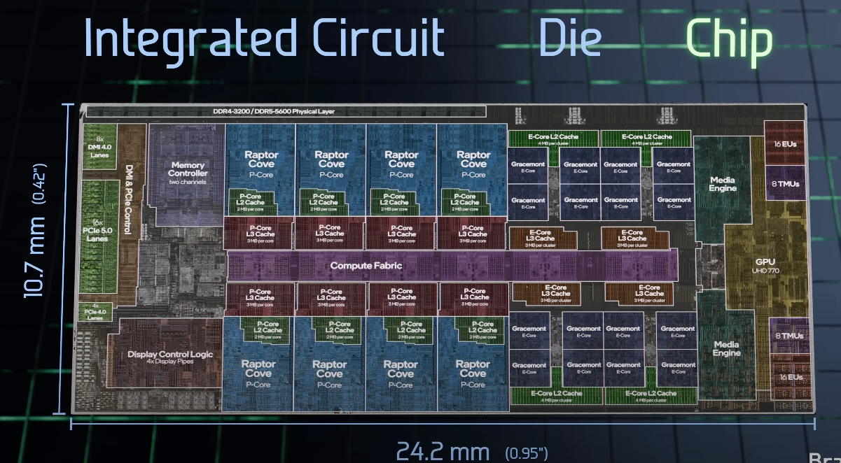
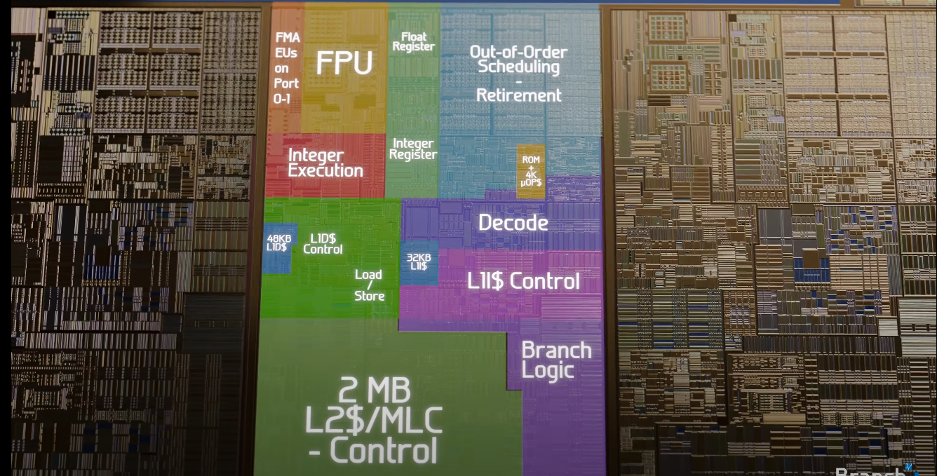
Intel Core i9-13900K labelled die shot. Source: How are Microchips Made?

To improve access speed, CPUs transfer data between main memory and cache in fixed-size chunks called cache lines or cache blocks. When a cache line is loaded from main memory, it is stored as a cache entry. For example, in AMD Ryzen Zen CPUs, the cache line size is 64 bytes. The cache takes advantage of data locality - how programs typically access memory. When a single floating-point number is requested from a continuous array in memory, the cache doesn’t just fetch that one value; it also preloads the next floating-point numbers and stores them in the cache. This is why reading data sequentially from an array is much more efficient than randomly accessing scattered memory locations. When the CPU needs to read or write to a memory location, it first checks if the data is already in the cache. This leads to two possible scenarios:

Cache Hit - If the requested memory location is found in the cache, the CPU can access it instantly, avoiding the need to fetch data from the much slower DRAM.
Cache Miss - If the requested data is not in the cache, the CPU retrieves it from the main memory and stores it in the cache for future access.

Since the cache has limited space, it must decide which data to replace when new information needs to be stored. This decision is governed by a cache replacement policy. Some of the most common policies include:

LRU (Least Recently Used): Replaces the cache entry that has gone unused the longest.
LFU (Least Frequently Used): Evicts the entry that has been accessed the least often.
LFRU (Least Frequently Recently Used): A hybrid approach that considers both recent and overall access frequency.

Similar to registers, once data is loaded into the cache, we want to reuse the data as much as possible to reduce main memory accesses. Given the cache’s limited capacity, storing entire input matrices $C, B, A$ in the cache isn’t feasible. Instead, we divide them into smaller blocks, load these blocks into the cache, and reuse them for rank-1 updates. This technique is often referred to as tiling or cache blocking, allowing us to handle matrices of arbitrary size effectively.

The single-threaded matrix multiplication with cache blocking can be visualized as shown in the image borrowed from the official BLIS repository:

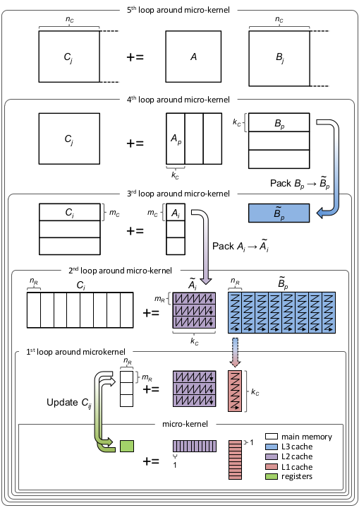
Let’s step through the diagram and discuss it. In the outer-most loop (5th loop) we iterate over dimension $N$, dividing matrix $C$ into blocks $C_j$ of size $M \times n_c$ and matrix $B$ into blocks $B_j$ of size $K \times n_c$. The subscript $c$ in $n_c$ stands for cache. In the 4th loop we iterate over dimension $K$ and divide matrix $A$ into $A_j$ of size $M \times k_c$ and $B_j$ into $B_p$ of size $k_c \times n_c$. Notice $B_p$ has fixed, limited size and can now be loaded into the cache. $B_p$ is packed into $\tilde{B}_p$, padded with zeros, if necessary, and loaded into the L3 cache. I In the 3rd loop we iterate over dimension $M$ and divide $C_j$ into $C_i$ (there is a typo in the diagram) of size $m_c \times n_c$ and $A_p$ into $A_j$ of size $m_c \times k_c$. Matrix $A_j$ is now restricted in size and can be loaded entirely into the L2 cache. $A_j$ is packed into $\tilde{A}_j$ and padded with zeros if needed. Note how we reuse the same $\tilde{B}_p$ block from the L3 cache for different $A_j$ blocks. Both $m_c$ and $n_c$ are chosen to be a multiple of $m_R$ and $n_R$ respectively.

In the last two loops we simply iterate over cached blocks and divide them into $m_R \times k_c$ and $k_c \times n_R$ panels. These panels are then passed to the kernel to perform rank-1 updates on the $m_R \times n_R$ sub-matrix of $C$, similarly to what we have already done in the previous chapter. Each panel of $\tilde{B}_p$ is loaded into the L1 cache and reused for multiple panels of $\tilde{A}_j$. Keep in mind that $\tilde{A}_j$ and $\tilde{B}_p$ are packed differently. During rank-1 updates we sequentially read a panel of $\tilde{A}_j$ column by column and a panel of $\tilde{B}_p$ row by row. Thus, each panel inside $\tilde{A}_j$ is stored in column-major order, while each panel inside $\tilde{B}_p$ is stored in row-major order.

Different CPU models have different cache sizes. To achieve peak performance, it’s crucial to optimize three key parameters: cache sizes for L1, L2, and L3 cashes (represented by $k_c$, $m_c$, and $n_c$ respectively). Theoretically, these parameters should be chosen so that:

$k_c \times n_c$ fills the entire L3 cache.
$m_c \times k_c$ fills the entire L2 cache.
$k_c \times n_R$ fills the entire L1 cache.

While these values provide a good starting point, using larger values often leads to better performance in practice. Unfortunately (or fortunately), we cannot manually place data into the cache or control which cache levels store the data; the CPU manages this automatically using cache replacement policies. Therefore, cache blocking and cache reuse must be implemented at the algorithm level through, for example, well-designed loops and strategic data access patterns.

The implementation matmul_cache.h straightforwardly follows the algorithm depicted in the diagram:

void matmul_cache(float* A, float* B, float* C, const int M, const int N, const int K) {
  for (int j = 0; j < N; j += NC) {
    const int nc = min(NC, N - j);
    for (int p = 0; p < K; p += KC) {
      const int kc = min(KC, K - p);
      pack_blockB(&B[j * K + p], blockB_packed, nc, kc, K);
      for (int i = 0; i < M; i += MC) {
        const int mc = min(MC, M - i);
        pack_blockA(&A[p * M + i], blockA_packed, mc, kc, M);
        for (int jr = 0; jr < nc; jr += NR) {
          for (int ir = 0; ir < mc; ir += MR) {
            const int mr = min(MR, mc - ir);
            const int nr = min(NR, nc - jr);
            kernel_16x6(&blockA_packed[ir * kc], &blockB_packed[jr * kc], &C[(j + jr) * M + (i + ir)], mr, nr, kc, M);
          }
        }
      }
    }
  }
}

8. Kernel Micro-Optimizations

Instead of using arrays of __m256 to define the accumulator $\bar{C}$ and the masks

__m256 C_buffer[6][2];
__m256i masks[2];

we explicitly unroll them

    __m256 C00 = _mm256_setzero_ps();
    __m256 C10 = _mm256_setzero_ps();
    __m256 C01 = _mm256_setzero_ps();
    __m256 C11 = _mm256_setzero_ps();
    __m256 C02 = _mm256_setzero_ps();
    __m256 C12 = _mm256_setzero_ps();
    __m256 C03 = _mm256_setzero_ps();
    __m256 C13 = _mm256_setzero_ps();
    __m256 C04 = _mm256_setzero_ps();
    __m256 C14 = _mm256_setzero_ps();
    __m256 C05 = _mm256_setzero_ps();
    __m256 C15 = _mm256_setzero_ps();
    __m256i packed_mask0;
    __m256i packed_mask1;

By doing this, GCC can better optimize the code avoiding register spilling. Additionally, we use vector instructions to calculate the masks as follows:

static int8_t mask[32]
    __attribute__((aligned(64))) = {-1, -1, -1, -1, -1, -1, -1, -1, -1, -1, -1, -1, -1, -1, -1, -1,
                                    0,  0,  0,  0,  0,  0,  0,  0,  0,  0,  0,  0,  0,  0,  0,  0};
packed_mask0 = _mm256_cvtepi8_epi32(_mm_loadu_si64(&mask[16 - mr]));
packed_mask1 = _mm256_cvtepi8_epi32(_mm_loadu_si64(&mask[16 - mr + 8]));

The corresponding implementation can be found at matmul_micro.h

9. Multithreading

There are indeed many loops that can be potentially parallelized. To achieve high-performance, we want to parallelize both packing and arithmetic operations. Let’s start with the arithmetic operations. The 5th, 4th, 3rd loops around the micro-kernel iterate over matrix dimensions in chunks of cache block sizes $n_c$, $k_c$, $m_c$. To efficiently parallelize the loops and keep all threads busy, we want number of iterations (=matrix dimension / cache block size) to be at least = number of threads (generally, the more the better). In other words, the input matrix dimension should be at least = number of threads * cache block size. As we discussed earlier, we also want cache blocks to fully occupy the corresponding cache levels. On modern CPUs, the second requirement results in cache block sizes of thousand(s) of elements. For example, on my Ryzen 9700X, cache block sizes of $n_c=1535$, $m_c=1024$ attain the best performance in the single-threaded scenario. Given the number of available cores on Ryzen 9700X, we need input matrices with dimensions of at least $\max(m_c, n_c) \times \text{number of cores} = 1535 \times 8 = 12280$ to be able to distribute the work over all cores.

In contrast, the last two loops iterate over cache blocks, dividing them into $m_R, n_R$ blocks. Since $n_R, m_R$ are typically very small (<20), these loops are ideal candidates for parallelization. Moreover, we can choose $m_c, n_c$ to be multiples of number of cores so that the work is evenly distributed across all cores.

On my machine, parallelizing the second and first inner loops jointly with collapse(2) results in the best performance:

#pragma omp parallel for collapse(2) num_threads(NTHREADS)
  for (int jr = 0; jr < nc; jr += NR)