Beating NumPy's matrix multiplication in 150 lines of C code
TL;DR
The code from the tutorial is available at matmul.c. This blog post is the result of my attempt to implement high-performance matrix multiplication on CPU while keeping the code simple, portable and scalable. The implementation follows the BLIS design, works for arbitrary matrix sizes, and, when fine-tuned for an AMD Ryzen 7700 (8 cores), outperforms NumPy (=OpenBLAS), achieving over 1 TFLOPS of peak performance across a wide range of matrix sizes.

By efficiently parallelizing the code with just 3 lines of OpenMP directives, it’s both scalable and easy to understand. The implementation hasn’t been tested on other CPUs, so I would appreciate feedback on its performance on your hardware. Although the code is portable and targets Intel Core and AMD Zen CPUs with FMA3 and AVX instructions (i.e., all modern Intel Core and AMD Zen CPUs), please don’t expect peak performance without fine-tuning the hyperparameters, such as the number of threads, kernel, and block sizes, unless you are running it on a Ryzen 7700(X). Additionally, on some Intel CPUs, the OpenBLAS implementation might be notably faster due to AVX-512 instructions, which were intentionally omitted here to support a broader range of processors. Throughout this tutorial, we’ll implement matrix multiplication from scratch, learning how to optimize and parallelize C code using matrix multiplication as an example. This is my first time writing a blog post. If you enjoy it, please subscribe and share it! I would be happy to hear feedback from all of you. This is the first part of my planned two-part blog series. In the second part, we will learn how to optimize matrix multiplication on GPUs. Stay tuned!
Intro
Matrix multiplication is an essential part of nearly all modern neural networks. For example, most of the time spent during inference in Transformers is actually taken up by matrix multiplications. Despite using matmul daily in PyTorch, NumPy, or JAX, I’ve never really thought about how it is designed and implemented to maximize hardware efficiency. To achieve such speeds, NumPy, for instance, relies on external BLAS (Basic Linear Algebra Subprograms) libraries. These libraries implement highly optimized common linear algebra operations such as dot product, matrix multiplication, vector addition, and scalar multiplication. Examples of BLAS implementations include:
- Intel MKL - optimized for Intel CPUs
- Accelerate - optimized for Apple CPUs
- BLIS - open-source, multi-vendor support
- GotoBLAS - open-source, multi-vendor support
- OpenBLAS - open-source, based on GotoBLAS
- etc.
If you look at the OpenBLAS code, you’ll notice it’s a mix of C and low-level assembly code. In fact, OpenBLAS, GotoBLAS, and BLIS are all written in C/FORTRAN/Assembly and contain matmul implementations handcrafted for different CPU types. During runtime, the appropriate function is called depending on the detected CPU device. I challenged myself and asked if it is possible to write a high-performance matmul (across a wide range of matrix sizes) without diving deep into Assembly and Fortran code, at least for my CPU. After some searching on the internet, I found a couple of exciting and educational step-by-step tutorials on how to implement fast matmul from scratch, covering both theoretical and practical aspects:
- Fast Multidimensional Matrix Multiplication on CPU from Scratch by Simon Boehm.
- Matrix Multiplication by Sergey Slotin.
- Geohot’s famous stream Can you multiply a matrix?
I highly recommend checking out these well-written and well-spoken tutorials with alternative matmul implementations. They helped me better understand the topic and, in some sense, motivated me to write a different implementation. Why? The reason is that all three solutions above work only for specific matrix sizes and do not achieve NumPy’s multi-threaded speed (except for Geohot’s implementation, which is comparable to NumPy in terms of speed but again works only for specific matrix sizes and requires an extra preswizzle step, resulting in a full copy of one of the input matrices). So, I wasn’t satisfied with the results and continued researching until I stumbled across two fascinating papers: “Anatomy of High-Performance Matrix Multiplication” and “Anatomy of High-Performance Many-Threaded Matrix Multiplication”. The former presents the BLAS implementation known as GotoBLAS, developed by Kazushige Goto. The latter briefly reviews the design of matmul op used in BLIS (an extended version of GotoBLAS) and discusses different parallelization possibilities for the matmul algorithm. After reading these papers I felt that the BLIS matmul design could potentially achieve all my goals:
- NumPy-like multi-threading performance across a broad range of matrix sizes
- Simple, portable and scalable C code
- Support for a wide variety of processors
In the next sections, we will implement the algorithm from the paper and compare it against NumPy.
NumPy Performance
By default, if installed via pip, numpy uses OpenBLAS on AMD CPUs. Therefore, throughout this tutorial I will use numpy and OpenBLAS interchangeably. Before performing any benchmarks, it’s always good practice to specify your hardware specs and development environment to ensure the results can be reproduced:
- CPU: Ryzen 7 7700 8 Cores, 16 Threads
- Freq: 3.8 GHz
- Turbo Freq: 5.3 GHz
- L1 Cache: 64 KB (per core)
- L2 Cache: 1MB (per core)
- L3 Cache: 32MB (shared), 16-way associative
- RAM: 32GB DDR5 6000 MHz CL36
- Numpy 1.26.4
- Compiler: clang-17
- Compiler flags:
-O2 -mno-avx512f -march=native - OS: Ubuntu 22.04.4 LTS
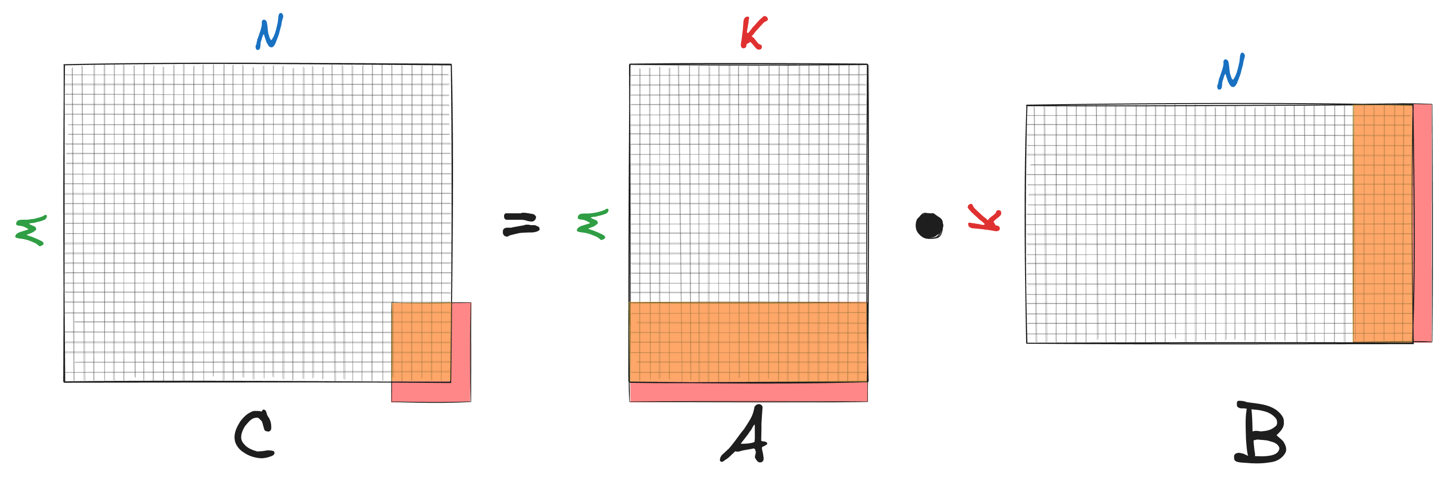
To multiply two float32 matrices A of shape \(M \times K\) and B of shape \(K \times N\), for each element of the resulting matrix C of shape \(M \times N\), we need to calculate the dot product between a row of A and a column of B. This results in \(K\) (additions) + \(K\) (multiplications) = \(2K\) FLoating Point Operations (FLOP) per element of matrix C or \(2KMN\) FLOP in total.
We will measure performance in terms of FLOP per second FLOP/s=FLOPS. In Python, this can be simply done as follows:
import numpy as np
import time

A = np.random.randn(M, K).astype(np.float32)
B = np.random.randn(K, N).astype(np.float32)
FLOP = 2*K*M*N

start = time.perf_counter()
C = A @ B
end = time.perf_counter()
exec_time = end - start
FLOPS = FLOP/exec_time
GFLOPS = FLOPS/1e9
Important! When benchmarking code, try to minimize the number of running tasks, especially when measuring multi-threaded code. Results obtained on Windows are usually lower than on Linux.
To benchmark numpy’s matmul, we will use benchmark_numpy.py, which executes the code snippet above for different matrix sizes in a loop and measures peak/average FLOPS. By default, numpy will use all available cores; however, we can easily change this by setting environment variables before importing numpy and matplotlib
os.environ["OPENBLAS_NUM_THREADS"] = "1"
os.environ["MKL_NUM_THREADS"] = "1"
os.environ["OMP_NUM_THREADS"] = "1"
import numpy as np
import matplotlib.pyplot as plt
To measure Numpy’s matmul performance, run
python benchmark_numpy.py -NITER=200 -ST -SAVEFIG
for single-threaded benchmark and
python benchmark_numpy.py -NITER=500 -SAVEFIG
for multi-threaded benchmark.
On my machine I got the following results:


How close are we to the theoretical upper limit achievable on the CPU?
Theoretical Limit
Recall the computer’s memory hierarchy (for now, ignore the layers between registers and RAM; we will discuss them later).

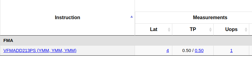
To perform arithmetic operations on data stored in RAM (off-chip memory, slow and large), the data must first be transferred to the CPU and eventually stored in CPU registers (on-chip memory, fast and small). Modern x86 CPUs support SIMD (Single Instruction Multiple Data) extensions, which allow multiple pieces of data to be processed in parallel. There are various SIMD extensions, but the ones relevant to our discussion are Advanced Vector Extensions (AVX) and Fused Multiply-Add (FMA). Both AVX and FMA operate on data stored in special 256-bit YMM registers. Each YMM register can hold up to 256/32 = 8 packed single-precision (32-bit) floats. The FMA extension allows a multiply-add operation to be performed in one step on data stored in YMM registers. The corresponding assembly instruction is called VFMADD213PS (PS stands for PackedSingle) and takes three registers (YMM1, YMM2, YMM3) as input to calculate YMM1 * YMM2 + YMM3 and store the result in YMM3, hence the “213” (there are also vfmadd132ps, vfmadd231ps variants).
According to the intel intrinsics guide or https://uops.info/table.html, the throughput (TP) of fused-multiply-add is 0.5 cycles/instruction or 2 instructions/cycle:
Theoretically, the CPU can execute 32 FLOP per cycle = 8 (floats in YMM register) * 2 (add + mul) * 2 (1/TP). On my machine, the CPU boosts up to 5.1 GHz in single-threaded tasks and up to 4.7 GHz in multi-threaded tasks. Therefore, a rough estimation of the maximum achievable FLOPS can be calculated as 5.1GHz * 32 FLOP/cycle = 163 GFLOPS for single-threaded matmul and 4.7GHz * 32 FLOP/cycle * 8 cores = 1203 GFLOPS for multi-threaded matmul. Starting from \(M=N=K=1000\), numpy reaches on average 92% of the theoretical maximum single-threaded performance and 85% of the multi-threaded. Can we compete with NumPy using plain C code without thousands of lines of low-level assembly code?
Naive Implementation
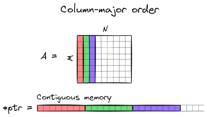
Without loss of generality in this implementation we will assume that matrices stored in column-major order. A matrix A of shape MxN is stored as contiguous array of length M*N and an element A[row][col] is accessed via C raw pointer ptr[col*M + row], where 0 <= col <= N-1 and 0 <= row <= M-1.
The naive implementation
can be implemented as follows:
void matmul_naive(float* A, float* B, float* C, const int M, const int N, const int K) {
  for (int i = 0; i < M; i++) {
    for (int j = 0; j < N; j++) {
      for (int p = 0; p < K; p++) {
        C[j * M + i] += A[p * M + i] * B[j * K + p];
      }
    }
  }
}
We iterate over all rows (first loop) and all columns (second loop) of the matrix C and for each element of C we calculate the dot product (third loop) between the corresponding rows and columns of matrices A and B. It’s always good to start with simple and robust implementation that can later be used to test optimized implementations for correctness. The file matmul_nave.c contains this implementation.
Running the naive implementation
clang-17 -O2 -mno-avx512f -march=native matmul_naive.c -o matmul_naive.out && ./matmul_naive.out
results in 2.7 GFLOPS on my machine. Nowhere near our target of 1 TFLOPS.
Kernel
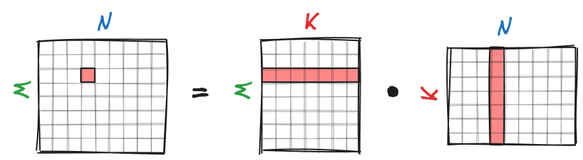
Matrix multiplication $C=AB$ can be decomposed into smaller sub-problems. The idea now is that if the smaller sub-problems can be solved quickly, then the entire matmul will be fast. We first partition the matrix $C$ of shape $M \times N$ into small sub-matrices of shape $m_R \times n_R$, where $n_R \ll N$ and $m_R \ll M$. To calculate $C=AB$, we iterate over $C$ and compute each of its $m_R \times n_R$ sub-matrices.
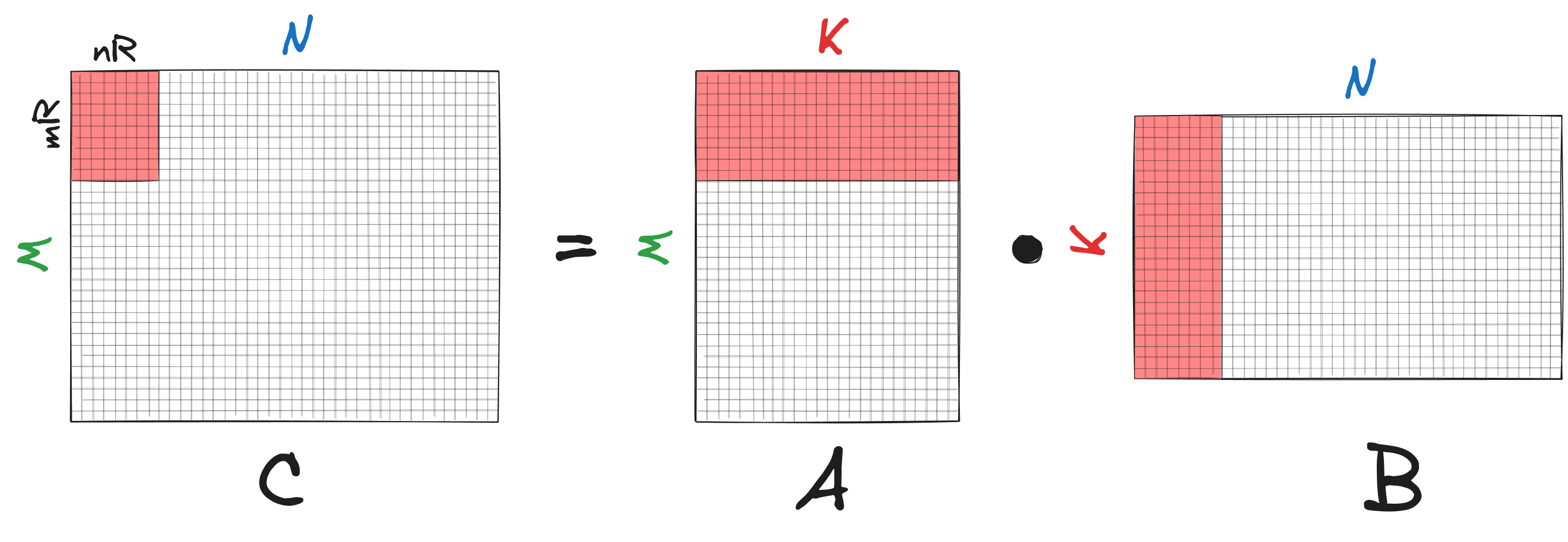
The function that calculates these tiny $m_R \times n_R$ sub-matrices $\bar{C}$ of $C$ is called a kernel or micro-kernel. This is the heart of high-performance matrix multiplication. When we say that a matmul algorithm is optimized for a particular CPU architecture, it often involves kernel optimization. For example, in the BLIS library, the kernels optimized for different processor types can be found under kernels.
Let’s take a closer look at the kernel.
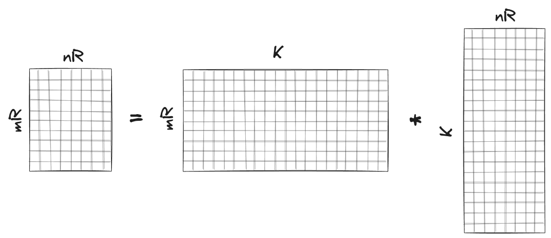
To calculate a $m_R \times n_R$ sub-matrix $\bar{C}$ of matrix $C$, we multiply matrix $\bar{A}$ of size $m_R \times K$ and matrix $\bar{B}$ of size $K \times n_R$. If we do this in a naive manner using dot products, we would need to fetch $2K$ (=dot product) elements from RAM to calculate a single element of $\bar{C}$ or $2K m_R n_R$ elements in total to calculate $\bar{C}$. However, there is an alternative strategy that can reduce the number of fetched elements.
We first load matrix $\bar{C}$ into SIMD (=YMM) registers (note that we can do this because both $n_R$ and $m_R$ are small). The subscript $R$ in $n_R$ and $m_R$ stands for “registers”. Then we iterate over $K$ and in each iteration we load 1 column of $\bar{A}$ and 1 row of $\bar{B}$ into YMM registers (again, note that both the row and the column vectors are small and fit in the registers). Finally, we perform matrix multiplication between the column and the row vectors to update the matrix $\bar{C}$. After $K$ iterations (=rank-1 updates), the matrix $\bar{C}$ is fully computed.
![]()
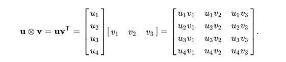
Example of matrix multiplication between a column and a row vector. Each column of the resulting matrix is computed by multiplying vector $\mathbf{u}$ with a scalar element of the row vector.
Overall we fetched $(m_R + n_R)K + m_R n_R \approx (m_R + n_R)K$ elements into registers. Compared to the naive strategy, we reduced the number by a factor of
\[\frac{2m_Rn_RK}{(m_R + n_R)K} = \frac{2m_Rn_R}{m_R + n_R}\]The factor is maximized when both $m_R$, $n_R$ are large and $m_R = n_R$. The values $m_R$ and $n_R$ are usually limited by the available memory in the registers.
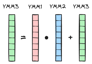
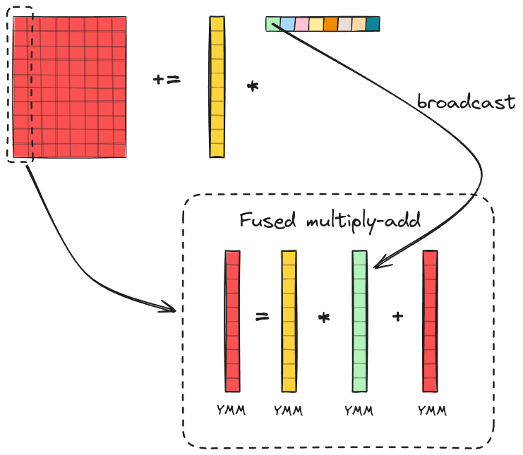
Now, let’s explore how a rank-1 update can be implemented using SIMD instructions. Each rank-1 update is a matrix multiplication between a column of $\bar{A}$ and a row of $\bar{B}$. Note how individual column of $\bar{C}$ is updated via scalar-vector multiplication between a column of $\bar{A}$ and a corresponding scalar element of a row of $\bar{B}$. Thanks to the FMA extension, the update + scalar-vector multiplication can be efficiently calculated via a fused multiply-add instruction. Before executing the FMA instruction, we only need to broadcast the scalar element of the row of $\bar{B}$ to a vector and load it into a YMM register. The parameter $m_R$ determines how many elements are stored in column vectors of $\bar{C}, \bar{A}$ and how many YMM registers we need for this. Since each YMM register can store up to 8 floats, we assume that $m_R$ is a multiple of 8 (8, 16, 24, 32…) and the elements in column vectors are packed into blocks of size 8. Then the number of YMM registers required to store the column vectors can be calculated as $m_R$ / 8. Note that we don’t need additional YMM registers for the broadcasted column vector of $\bar{B}$ since the same 8-float vector (YMM Register) can be reused to update all 8-float blocks of the column vector of $\bar{C}$.
Thus, the complete algorithm for a single rank-1 update of the matrix $\bar{C}$ is as follows:
- Load matrix $\bar{C}$ into YMM registers
- Load the column vector of matrix $\bar{A}$
- Set n = 1
- Load the n-th scalar element of the row of $\bar{B}$, broadcast it to a vector and place it into YMM register.
- Update the n-th column of $\bar{C}$ via fused matrix multiply
- Increment n by 1.
- Repeat steps 4-6 until all columns of $\bar{C}$ are updated.
The last thing we need to discuss before implementing the kernel in C is how to choose the kernel size = $m_R$ and $n_R$. CPUs that support AVX instructions have 16 YMM registers. From our previous observations, we know that we need $n_R m_R / 8$ registers to store the matrix $\bar{C}$, $m_R/8$ registers to store the column vector of $\bar{A}$ and 1 register for the broadcasted vector of $\bar{B}$. We want $m_R, n_R$ as large as possible and satisfying the following conditions
- $n_R m_R/8 + m_R/8 + 1 <= 16$
- $m_R$ is a multiple of 8
In theory we also want $m_R \approx n_R$ to minimize the number of fetched elements. However, in practice, I’ve found out that the non-square $m_R \times n_R= 16 \times 6$ kernel shows the best results on my machine. You are free to try out different kernel sizes, for example, $8 \times 12$, $8 \times 13$, $8 \times 14$ and compare the performance on your CPU.
Let’s implement the $16 \times 6$ kernel in C. The code can be found in matmul_kernel.c. To use the SIMD instructions we need to include the immintin.h library.
#include <immintrin.h>
the kernel function is declared as follows:
void kernel_16x6(float* A, float* B, float* C, const int M, const int N, const int K);
The function takes as input 3 matrices + their dimensions and calculates a $16\times6$ sub-matrix $\bar{C}$ of $C$. Inside the function, first, declare the variables that reside in YMM registers:
__m256 C_buffer[2][6];
__m256 b_packFloat8;
__m256 a0_packFloat8;
__m256 a1_packFloat8;
The __m256 datatype is a vector of 8 floats (8x32 = 256 bits) that resides in YMM register. C_buffer is a 16x6 sub-matrix of $C$ stored in YMM registers. The first dimension of C_buffer is 2, because we need 16/8=2 registers to store 16 elements. b_packFloat8, a0_packFloat8, a1_packFloat8 are column vectors of $\bar{B}$ and $\bar{A}$. Again, we need two vectors to store 16 elements of the column vector of $\bar{A}$.
Next, we load the sub-matrix $\bar{C}$ into YMM registers:
for (int j = 0; j < 6; j++) {
  C_buffer[0][j] = _mm256_loadu_ps(&C[j * M]);
  C_buffer[1][j] = _mm256_loadu_ps(&C[j * M + 8]);
}
SIMD C functions are well documented and can be found in the Intel Intrinsics Guide. For example, _mm256_loadu_ps

In the next step, we iterate over K and, in each iteration, load a column vector of $\bar{A}$, broadcast a scalar value of $\bar{B}$ to a vector, and perform a fused multiply-add operation to update 1 column of C_buffer:
for (int p = 0; p < K; p++) {
  a0_packFloat8 = _mm256_loadu_ps(&A[p * M]);
  a1_packFloat8 = _mm256_loadu_ps(&A[p * M + 8]);
  b_packFloat8 = _mm256_broadcast_ss(&B[p]);
  C_buffer[0][0] = _mm256_fmadd_ps(a0_packFloat8, b_packFloat8, C_buffer[0][0]);
  C_buffer[1][0] = _mm256_fmadd_ps(a1_packFloat8, b_packFloat8, C_buffer[1][0]);
  ...
}
Then repeat the step for the remaining 5 columns. We manually unroll the loop when updating 6 columns of C_buffer so that clang can optimize the code.
Finally, we write the sub-matrix C_buffer back to C:
for (int j = 0; j < 6; j++) {
  _mm256_storeu_ps(&C[j * M], C_buffer[0][j]);
  _mm256_storeu_ps(&C[j * M + 8], C_buffer[1][j]);
}
To perform matrix multiplication, we simply iterate over the matrix $C$ and apply the kernel to it’s sub-matrices:
#define MR 16
#define NR 6

void matmul_kernel(float* A, float* B, float* C, const int M, const int N, const int K) {
  assert(M % MR == 0);
  assert(N % NR == 0);
  for (int i = 0; i < M; i += MR) {
    for (int j = 0; j < N; j += NR) {
        kernel_16x6(&A[i], &B[j * K], &C[j * M + i], M, N, K);
    }
  }
}
The new implementation
clang-17 -O2 -mno-avx512f -march=native -DTEST -DNITER=100 matmul_kernel.c -o matmul_kernel.out && ./matmul_kernel.out
results in 147 GFLOPS - a gigantic gain compared to the initial 2.7 GFLOPS. Additionally, we can check the assembly code produced by the compiler via
clang-17 -O2 -mno-avx512f -march=native matmul_kernel.c -S > matmul_kernel.txt
to ensure that the SIMD instructions and the YMM registers are utilized:
vbroadcastss	(%rsi,%rbp,4), %ymm14
vbroadcastss	(%rbx,%rbp,4), %ymm15
vfmadd231ps	%ymm14, %ymm12, %ymm3   # ymm3 = (ymm12 * ymm14) + ymm3
vfmadd231ps	%ymm14, %ymm13, %ymm1   # ymm1 = (ymm13 * ymm14) + ymm1
vbroadcastss	(%r13,%rbp,4), %ymm14
vfmadd231ps	%ymm12, %ymm15, %ymm11  # ymm11 = (ymm15 * ymm12) + ymm11
vfmadd231ps	%ymm15, %ymm13, %ymm10  # ymm10 = (ymm13 * ymm15) + ymm10
vfmadd231ps	%ymm14, %ymm12, %ymm2   # ymm2 = (ymm12 * ymm14) + ymm2
vfmadd231ps	%ymm14, %ymm13, %ymm0   # ymm0 = (ymm13 * ymm14) + ymm0
vbroadcastss	(%r12,%rbp,4), %ymm14
vfmadd231ps	%ymm14, %ymm12, %ymm5   # ymm5 = (ymm12 * ymm14) + ymm5
vfmadd231ps	%ymm14, %ymm13, %ymm4   # ymm4 = (ymm13 * ymm14) + ymm4
vbroadcastss	(%r15,%rbp,4), %ymm14
vfmadd231ps	%ymm14, %ymm12, %ymm7   # ymm7 = (ymm12 * ymm14) + ymm7
vfmadd231ps	%ymm14, %ymm13, %ymm6   # ymm6 = (ymm13 * ymm14) + ymm6
vbroadcastss	(%r14,%rbp,4), %ymm14
vfmadd231ps	%ymm14, %ymm12, %ymm9   # ymm9 = (ymm12 * ymm14) + ymm9
vfmadd231ps	%ymm14, %ymm13, %ymm8   # ymm8 = (ymm13 * ymm14) + ymm8
Masking And Packing
You might notice that the current kernel implementation works only for matrix sizes that are multiples of $m_R$ and $n_R$. To make the algorithm work for arbitrary matrix sizes, we need to handle edge cases where the kernel doesn’t fully overlap with matrix $C$.
First of all, we when loading and storing the elements of $C$, we should pick the elements only within the matrix boundary. The case where the number of overlapped columns $n$ is less than $n_R$ is straightforward - we simply iterate over $n$ columns within the $C$ boundary:
# n - number of overlapped columns within C boundary

# "j<n" instead "j<6", since n can be less than 6.
for (int j = 0; j < n; j++) {
  C_buffer[0][j] = _mm256_loadu_ps(&C[j * M]);
  C_buffer[1][j] = _mm256_loadu_ps(&C[j * M + 8]);
}
Handling the case where the number of overlapped rows $m$ differs from $m_R$ is a bit trickier because _mm256_loadu_ps loads 8 elements at once. Fortunately, there is a function called _mm256_maskload_ps which loads 8 floats based on mask bits associated with each data element. It takes as input 2 arguments: const float* data and __m256i mask. __m256i is a 256-bit vector of 8x32-bit integers. The most significant bit (MSB) of each integer represents the mask bits. If a mask bit is zero, the corresponding value in the memory location is not loaded and the corresponding field in the return value is set to zero. For example, MSB of unsigned integer 2147483648 (binary representation 10000000 00000000 00000000 00000000) is 1, hence corresponding float in data will be loaded. On the other hand, MSB of unsigned integer 2147483647 (binary format 01111111 11111111 11111111 11111111) is 0, hence the corresponding float in data will not be loaded. The function _mm256_maskstore_ps works similarly, except it stores data instead of loading.
If $m \neq m_R$ , we create integer masks by left-shifting the unsigned integer 65535 (=00000000 00000000 11111111 111111111 in binary format) depending on the number of overlapped rows $m$. The function _mm256_setr_epi32 creates an 8-integer vector from 8 32-bit integers.
__m256i masks[2];
if (m != MR) {
  const unsigned int bit_mask = 65535;
  masks[0] = _mm256_setr_epi32(bit_mask << (m + 15), bit_mask << (m + 14),
                 bit_mask << (m + 13), bit_mask << (m + 12),
                 bit_mask << (m + 11), bit_mask << (m + 10),
                 bit_mask << (m + 9), bit_mask << (m + 8));
  masks[1] = _mm256_setr_epi32(bit_mask << (m + 7), bit_mask << (m + 6),
                 bit_mask << (m + 5), bit_mask << (m + 4),
                 bit_mask << (m + 3), bit_mask << (m + 2),
                 bit_mask << (m + 1), bit_mask << m);

  for (int j = 0; j < n; j++) {
    C_buffer[0][j] = _mm256_maskload_ps(&C[j * M], masks[0]);
    C_buffer[1][j] = _mm256_maskload_ps(&C[j * M + 8], masks[1]);
  }
}
The same masks are used to store the results back after rank-1 updates.
Additionally, we copy and pad with zeros (if needed) $m \times K$, $K \times n$ blocks of $A$ and $B$ into arrays with static shapes $m_R \times K$, $n_R \times K$.
void pack_blockA(float* A, float* blockA_packed, const int m, const int M,
                 const int K) {
  for (int p = 0; p < K; p++) {
    for (int i = 0; i < m; i++) {
      *blockA_packed = A[p * M + i];
      blockA_packed++;
    }
    for (int i = m; i < MR; i++) {
      *blockA_packed = 0.0;
      blockA_packed++;
    }
  }
}
These blocks with static shapes are then passed into the kernel, so that the rank-1 update inside the kernel can remain unchanged and be optimized during compilation time.
void matmul_pack_mask(float* A, float* B, float* C, float* blockA_packed,
                        float* blockB_packed, const int M, const int N,
                        const int K) {
  for (int i = 0; i < M; i += MR) {
    const int m = min(MR, M - i);
    pack_blockA(&A[i], blockA_packed, m, M, K);
    for (int j = 0; j < N; j += NR) {
      const int n = min(NR, N - j);
      pack_blockB(&B[j * K], blockB_packed, n, N, K);
      kernel_16x6(blockA_packed, blockB_packed, &C[j * M + i], m, n, M, N, K);
    }
  }
}
The new implementation matmul_cache.c achieves “only” 56 GFLOPS on my machine:
clang-17 -O2 -mno-avx512f -march=native -DTEST -DNITER=100 matmul_pack_mask.c -o matmul_pack_mask.out && ./matmul_pack_mask.out
We see roughly a 2.6x decrease in performance, mostly because of frequently copying large $K$ dimensional sub-matrices of $A$ and $B$ from main memory. For each $m_R \times K$ sub-matrix of $A$ the entire(!) matrix $B$ is copied. Let’s optimize data reuse and cache management to finally achieve numpy’s level of performance for arbitrary matrix sizes.
Caching
Recall the CPU’s memory system diagram. Initially, we’ve ignored the intermediate layer between main-memory (DRAM) and the CPU’s registers - the CPU Cache.

Unlike DRAM, the cache is on-chip memory used to store frequently and recently accessed data from main memory. This minimizes data transfers between main memory and registers. Although faster than DRAM, the cache has limited capacity. CPUs typically employ a multi-level cache hierarchy for efficient data access. Levels like L1, L2, and L3 offer progressively larger capacities but slower access times, with L1 being the fastest and closest to the core.
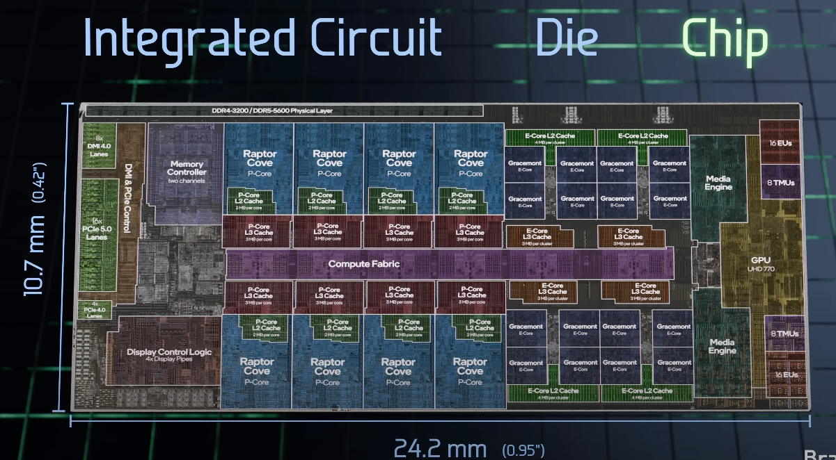
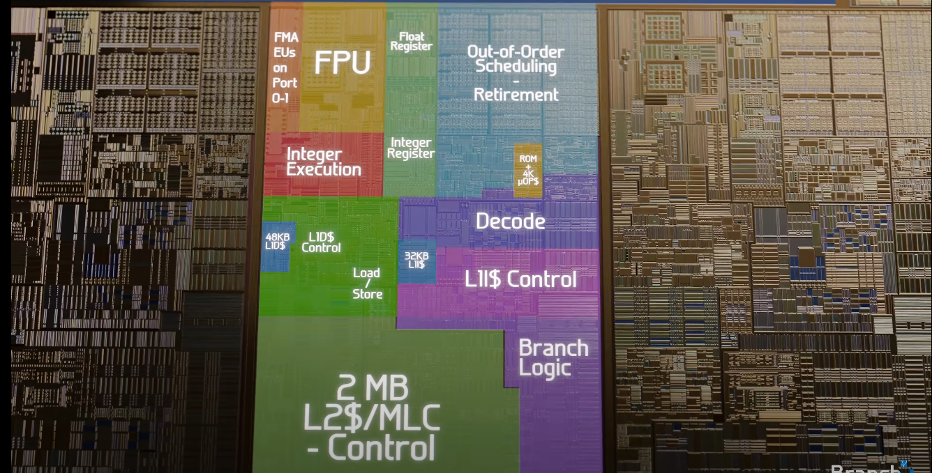 Intel Core i9-13900K labelled die shot. Source: How are Microchips Made?
To enhance access speed, CPUs transfer data between main memory and cache in fixed-size chunks called cache lines or cache blocks. When a cache line is transferred, a corresponding cache entry is created to store it. On Ryzen 7700, the cache line size is 64 bytes. The cache takes advantage of how we typically access data. When a single floating-point number from a continuous array in memory is requested, the cache cleverly grabs the next 15 floats along the way and stores them as well. This is why reading data sequentially from a contiguous array is much faster than jumping around to random memory locations. When the processor needs to read or write to a memory location, it first checks the cache for a corresponding entry. If the processor finds the memory location in the cache, a cache hit occurs. However, if the memory location is not found in the cache, a cache miss occurs. In the case of a cache miss, the cache allocates a new entry and copies the data from main memory. If the cache is full, a cache replacement policy kicks in to determine which data gets evicted to make room for new information. Several cache replacement policies exist, with LRU (Least Recently Used), LFU (Least Frequently Used), and LFRU (Least Frequently Recently Used) being the most widely used.
Similar to registers, once data is loaded into the cache, we want to reuse the data as much as possible to reduce main memory accesses. Given the cache’s limited capacity, storing entire input matrices input matrices $C, B, A$ in the cache isn’t feasible. Instead, we divide them into smaller blocks, load these blocks into the cache, and reuse them for rank-1 updates. This technique is often referred to as tiling or cache blocking, allowing us to handle matrices of arbitrary size effectively.
The final single-threaded matrix multiplication implementation, including the cache blocking, can be visualized as shown in the image borrowed from the official BLIS repository:
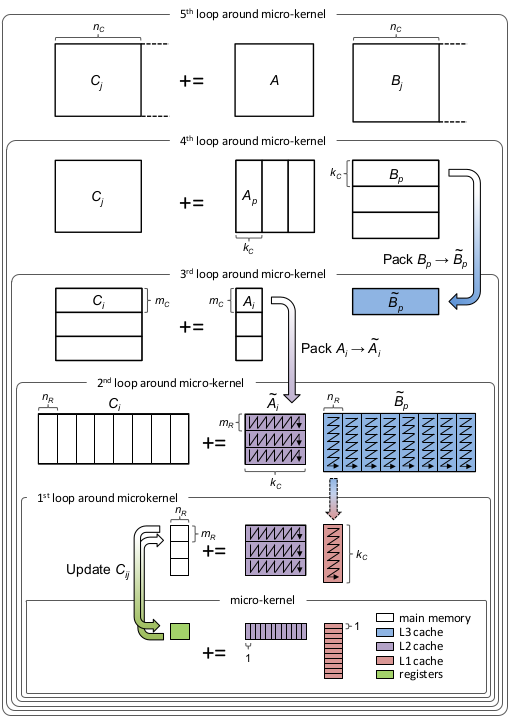
Let’s step through the diagram and discuss it. In the outer-most loop (5th loop) we iterate over dimension $N$, dividing matrix $C$ into blocks $C_j$ of size $M \times n_c$ and matrix $B$ into blocks $B_j$ of size $K \times n_c$. The subscript $c$ in $n_c$ stands for cache. In the 4th loop we iterate over dimension $K$ and divide matrix $A$ into $A_j$ of size $M \times k_c$ and $B_j$ into $B_p$ of size $k_c \times n_c$. Notice $B_p$ has fixed, limited size and can now be loaded into the cache. $B_p$ is packed into $\tilde{B}_p$, padded with zeros, if necessary, and loaded into the L3 cache. I In the 3rd loop we iterate over dimension $M$ and divide $C_j$ into $C_i$ (there is a typo in the diagram) of size $m_c \times n_c$ and $A_p$ into $A_j$ of size $m_c \times k_c$. Matrix $A_j$ is now restricted in size and can be loaded entirely into the L2 cache. $A_j$ is packed into $\tilde{A}_j$ and padded with zeros if needed. Note how we reuse the same $\tilde{B}_p$ block from the L3 cache for different $A_j$ blocks. Both $m_c$ and $n_c$ are chosen to be a multiple of $m_r$ and $n_r$ respectively.
In the last two loops we simply iterate over cached blocks and divide them into $m_R \times k_c$ and $k_c \times n_R$ panels. These panels are then passed to the kernel to perform rank-1 updates on the $m_R \times n_R$ sub-matrix of $C$, similarly to what we have already done in the previous chapter. Each panel of $\tilde{B}_p$ is loaded into the L1 cache and reused for multiple panels of $\tilde{A}_j$. Keep in mind that $\tilde{A}_j$ and $\tilde{B}_p$ are packed differently. During rank-1 updates we sequentially read a panel of $\tilde{A}_j$ column by column and a panel of $\tilde{B}_p$ row by row. Thus, each panel inside $\tilde{A}_j$ is stored in column-major order, while each panel inside $\tilde{B}_p$ is stored in row-major order.
Different CPU models have varying cache sizes. To achieve peak performance, it’s crucial to optimize three key parameters: cache sizes for L1, L2, and L3 cashes (represented by $k_c$, $m_c$, and $n_c$ respectively). Theoretically, these parameters should be chosen so that:
- The matrix $k_c \times n_c$ fills the entire L3 cache.
- The matrix $m_c \times k_c$ fills the entire L2 cache.
- The matrix $k_c \times n_R$ fills the entire L1 cache.
While these values provide a good starting point, using larger values often leads to better performance in practice. Unfortunately (or fortunately), we cannot manually place data into the cache or control which cache levels store the data; the CPU manages this automatically using cache replacement policies. Therefore, cache blocking and cache reuse must be implemented at the algorithm level through, for example, well-designed loops and strategic data access patterns.
The implementation straightforwardly follows the algorithm depicted in the diagram:
void matmul_cache(float* A, float* B, float* C, const int M, const int N,
                  const int K) {
  for (int j = 0; j < N; j += NC) { // 5th loop
    const int nb = min(NC, N - j);
    for (int p = 0; p < K; p += KC) { // 4th loop
      const int kb = min(KC, K - p);
      pack_blockB(&B[j * K + p], blockB_packed, nb, kb, K);
      for (int i = 0; i < M; i += MC) { // 3rd loop
        const int mb = min(MC, M - i);
        pack_blockA(&A[p * M + i], blockA_packed, mb, kb, M);
        for (int jr = 0; jr < nb; jr += NR) { // 2nd loop
          const int nr = min(NR, nb - jr);
          for (int ir = 0; ir < mb; ir += MR) { // 1st loop
            const int mr = min(MR, mb - ir);
            kernel_16x6(&blockA_packed[ir * kb], &blockB_packed[jr * kb],
                        &C[(j + jr) * M + (i + ir)], mr, nr, kb, M);
          }
        }
      }
    }
  }
}
Before implementing the multi-threaded version of the algorithm, let’s benchmark our current implementation and compare it against numpy:
python benchmark_numpy.py -ST

clang-17 -O2 -mno-avx512f -march=native benchmark_st.c -o benchmark_st.out && ./benchmark_st.out

python plot_benchmark.py

Multithreading
There are indeed many loops that can be potentially parallelized. To achieve high-performance, we want to parallelize both packing and arithmetic operations. Let’s start with the arithmetic operations. The 5th, 4th, 3rd loops around the micro-kernel iterate over matrix dimensions in chunks of cache block sizes $n_c$, $k_c$, $m_c$. To efficiently parallelize the loops and keep all threads busy, we want number of iterations (=matrix dimension / cache block size) to be at least = number of threads (generally, the more the better). In other words, the input matrix dimension should be at least = number of threads * cache block size. As we discussed earlier, we also want cache blocks to fully occupy the corresponding cache levels. On modern CPUs, this second requirement results in cache block sizes of thousand(s) of elements. For example, on my Ryzen 7700, cache block sizes of $n_c=1535$, $m_c=1024, k_c=2000$ attain the best performance in the single-threaded case. Given the number of available threads on Ryzen 7700, $Nthreads=16$, we need input matrices with dimensions of at least $2000 \times 16$ to be able to distribute the work over all threads.
In contrast, the last two loops iterate over cache blocks, dividing them into $m_r, n_r$ blocks. Since $n_r, m_r$ are typically very small (<20), these loops are ideal candidates for parallelization. Moreover, we can choose $m_c, n_c$ to be multiples of $Nthreads$ so that the work is evenly distributed across all threads.
On my machine, parallelizing the second loop results in much better performance compared to the first loop (possibly due to large $n_c$ and little work in each iteration of the first loop). We will therefore parallelize the second loop using OpenMP directives (more on OpenMP here, here and here):
#pragma omp parallel for num_threads(NTHREADS) schedule(static)
  for (int jr = 0; jr < nb; jr += NR)
It’s also possible to parallelize the 2nd and 1st loops using
#pragma omp parallel for collapse(2), which leads to similar performance when parallelizing only the 2nd loop.
Together with arithmetic operations, we also want to accelerate the packing of both $\tilde{A}$ and $\tilde{B}$:
void pack_blockA(float* A, float* blockA_packed, const int mb, const int kb, const int M)
#pragma omp parallel for num_threads(NTHREADS) schedule(static)
  for (int i = 0; i < mb; i += MR)
void pack_blockB(float* B, float* blockB_packed, const int nb, const int kb, const int K)
#pragma omp parallel for num_threads(NTHREADS) schedule(static)
  for (int j = 0; j < nb; j += NR)
Similar to arithmetic operations, the packing loops can be easily parallelized due to the high number of iterations and the flexibility of choosing $m_c, k_c, n_c$.
Running
clang-17 -O2 -mno-avx512f -march=native -DNITER=100 -fopenmp matmul_parallel.c -o matmul_parallel.out && ./matmul_parallel.out
shows around 1 TFLOPS. Don’t forget to add the -fopenmp compiler flag to use OpenMP directives. You might also need to install libomp-dev with sudo apt install libomp-dev.
Let’s check the CPU utilization
htop

and benchmark the multithreading implementation:
python benchmark_numpy.py
clang-17 -O2 -mno-avx512f -march=native -fopenmp benchmark_mt.c -o benchmark_mt.out && ./benchmark_mt.out
python plot_benchmark.py